Fluorescence and fluorescence lifetime
Molecules contain several single energy states S0, S1, S2... and triplet states T1..., each of which contains several fine energy levels. Under normal circumstances, most of the electrons are in the *low energy state, i.e., the *low energy level of the ground state S0. When the molecule is irradiated by a beam of light, it will absorb the photon energy, and the electrons will be excited to the higher energy states S1 or S2, and the electrons in the S2 energy state will only be present for a very short period of time, and then they will jump to S1 through the process of internal conversion, while the electrons in the S1 energy state will jump to the *low energy level of S1 in a very short time, and the electrons will exist for a period of time, and then will be excited through the process of quaking. These electrons will exist for some time and then migrate to the ground state by oscillatory relaxation radiation, a process that releases a photon, i.e., fluorescence.
In addition, there is also a jump of electrons to the triplet state T1 and then from T1 to the ground state, which we call phosphorescence.

Fluorescent properties
When studying fluorescence properties, the following aspects are mainly analyzed: excitation spectrum, emission spectrum, fluorescence intensity, polarized fluorescence, fluorescence luminescence quantum yield, fluorescence lifetime and so on. Among them, Fluorescence Lifetime is the average time (nanoseconds) that a fluorescent molecule exists in the excited state.
Fluorescence Life Test
Fluorescence lifetimes are typically between a few nanoseconds and a few hundred nanoseconds, and today there are two main types of test methods: time-domain measurements and frequency-domain measurements of time-stability experimental test curves:
1 Time-domain measurements
A narrow pulse excites a fluorescent molecule to a higher energy state S1, followed by a measurement of the change in fluorescence emission probability with time. One of the most widely used is time correlated single photon counting, TCSPC (Time Correlated Single Photon Counting).
Time Correlated Single Photon Counting (TCSPC) enables transient testing from hundreds of ps-ns-us, a method that relies solely on fast detectors and high-speed circuitry for data acquisition. The time difference between the *one* (and only) photon emitted by the sample after excitation and the excitation light is statistically counted, i.e., the time difference between the START moment and the STOP moment in the figure below. Due to the requirement of Stop signal, TCSPC generally needs a high repetition frequency light source as the excitation source, the repetition of which should be at least above 100KHz, and most of the light sources will reach the MHz level; at the same time, in general, we also need to control the number of Stop signals, so as to satisfy the requirement that the sample generates and only generates an effective fluorescence signal of one photon in one excitation cycle, avoiding the emergence of photon pairs. In addition, the number of Stop signals should be controlled so that the sample produces only one photon of effective fluorescence signal in one excitation cycle.

2 Frequency Domain Measurements
After amplitude modulation of the continuous excitation light, the fluorescence intensity emitted by the molecule is also amplitude modulated, and there is a phase difference between the two modulation signals that is related to the fluorescence lifetime, and therefore this phase difference can be measured to calculate the fluorescence lifetime.

The left figure shows the frequency domain display of sinusoidally modulated excitation light (green) and the corresponding phase change frequency domain display of the emitted light signal (red).
The right figure shows the frequency domain display of modulation and phase corresponding to different lifetimes.TM- modulation lifetime, TP- phase lifetime. [1]
Fluorescence Lifetime Imaging for Microscopy (FLIM)
Fluorescence Lifetime ImagingMicroscopy (FLIM) is a technique to show the spatial distribution of fluorescence lifetimes at the microscopic scale, which is currently an important characterization and measurement tool in the fields of biomedical engineering, optoelectronic semiconductor materials, and so on, due to its irreversible influence of the concentration of the sample and its excellent performance that cannot be replaced by other fluorescence imaging techniques. an important characterization and measurement tool.
FLIM is generally categorized into wide field FLIM and laser scanning FLIM.

Wide Field FLIM (WFM)
The technique involves illuminating the sample with parallel light and focusing it with an objective lens to obtain a fluorescence signal, which is then captured by a wide-field camera. Wide-field FLIM is often used to quickly acquire images of large sample areas. Either time or frequency domain lifetime acquisitions can be applied to wide field imaging FLIM. Wide field FLIM has the advantage of higher frame rates and lower damage.

2 Laser Scanning FLIM (LSM)
Laser scanning FLIM acquires the fluorescence decay curves of a sample point by point over a selected area and then fits them to synthesize a fluorescence lifetime image. Compared with wide-field FLIM, it has greater advantages in spatial resolution and signal-to-noise ratio. There are two types of scanning methods: one with a fixed sample and a moving laser, and one with a fixed laser and a motorized displacement stage moving the sample.

FLIM Applications
Materials Science
- Lesson-lifetime mapping measurements of wide-band semiconductors such as GaN, SiC, etc.
- Quantum dots such as CdSe@ZnS as fluorescence lifetime imaging microscopy probes
- Component Analysis, Defect Detection of Chalcogenide Battery/LED Thin Film
- Detection of components and defects in copper indium gallium selenide CIGS and copper zinc tin sulfur CZTS thin film solar cells
- Lanthanide upconversion nanoparticles
- Carrier diffusion studies in GaAs or GaAsP quantum wells
Life Sciences
- Analysis of cell body autofluorescence lifetimes
- Effective differentiation of autofluorescence relative to fluorescent labeling
- Measurement of the pH value of the aqueous medium in living cells
- Local Oxygen Concentration Measurement
- Differentiation of different fluorescent markers with the same spectral properties
- Measurement of intracellular calcium concentration in living cells
- Time-resolved resonance energy transfer (FRET): far-off measurements on the nanoscale, quantitative measurements with environmentally sensitive FRET probes
- Metabolic imaging: fluorescence lifetime imaging of NAD(P)H and FAD cytoplasmic bodies
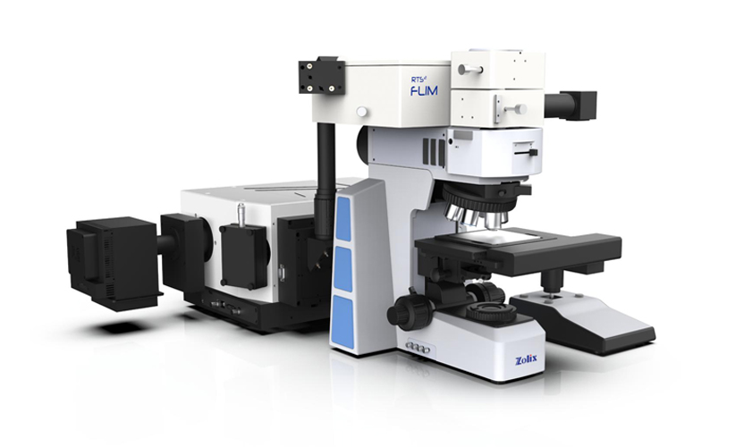
OmniFluo-FLIMMicrofluorescence Lifetime Imaging System Application Examples
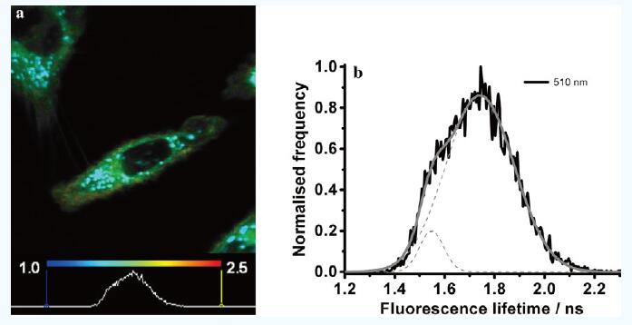
1 Staining of Hela cells with fluorescent molecules
Staining of Hela cells (a type of cervical cancer cells) with the fluorescent molecular rotor Bodipy-C12.
(a) Microscopic fluorescence lifetime imaging plot with lifetimes ranging from 1 ns (blue) to 2.5 ns (red);
(b) Histogram of fluorescence lifetimes, with short lifetimes around 1.6 ns for fat droplets and longer lifetimes around 1.8 ns for other locations in the cell.
Time-resolved measurements with fluorescent molecular rotors* have the great advantage that fluorescence lifetimes have sufficiently clear labeling properties and are independent of fluorophore concentration. [2]
2 Metal-modified fluorescence
Metal-modified fluorescence:
(a) Fluorescence lifetime as a function of the distance from the fluorophore to the gold surface;
(b) Confocal xz cross-section of a cell membrane of a breast adenocarcinoma cell labeled with green fluorescent protein (GFP), vertical scale bar: 5m;
(c) FLIM plot of b plot with shortened GFP fluorescence lifetime near the gold surface. [2]

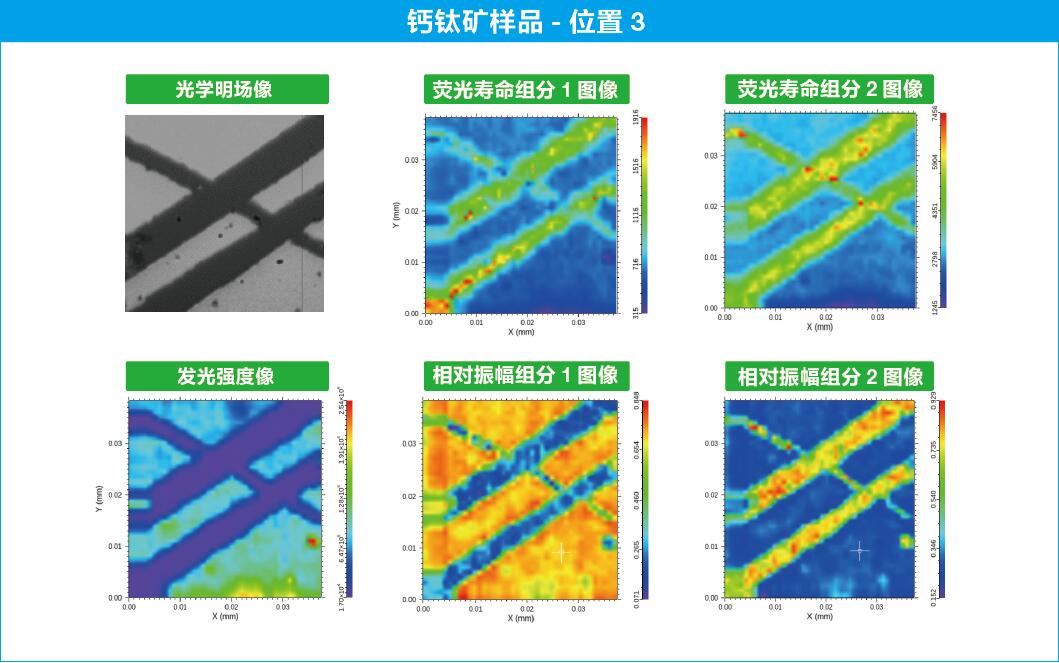
3 Chalcogenide solar cells
In the study below, a dynamic hot air (DHA) preparation process is demonstrated to control the film morphology and stability of fully inorganic PSCs, which does not contain conventional hazardous anti-solvents and can be prepared in an atmospheric environment. Meanwhile, the chalcogenides are doped with barium (Ba2+) alkali metal ions (BaI2:CsPbI2Br). This DHA method helps to form homogeneous grains and control crystallization, resulting in stable, all-inorganic PSCs. thus forming a complete black phase under ambient conditions. The DHA-treated chalcogenide PV devices have an efficiency of 14.851 TP2T for a small area of 0.09 cm and a *high* efficiency of 13.781 TP2T for a large area of 1x1 cm.The devices prepared by the DHA method still maintain the initial efficiency of 921 TP2T after 300h.

4 Multi-quantum well studies of MQWs
Confocal PL mapping images of MQWs grown on (a) sapphire and (b) GaN. A *higher density of luminescent clusters with smaller sizes is observed for MQWs grown on GaN. confocal TRPL mapping images of MQWs grown on (c) sapphire and (d) GaN. Only for MQWs grown on GaN, the region of strong PL intensity matches well with the region of longer PL decay time. Localized PL decay curves measured at points A and B for MQWs grown on (e) sapphire and (f) GaN, both labeled in the figure. For MQWs grown on GaN, the PL decay time difference between points A and B is higher.

OmniFluo-FLIMrangeMicrofluorescence Lifetime Imaging System Parameter Configuration
The microscopic fluorescence lifetime imaging system provided by Beijing ZhuoLi HanKuang Instrument Co., Ltd. is based on the microscopic and time-dependent single photon counting technology, together with the high-precision displacement stage to get the fluorescence decay curves of each spatial distribution point on the surface of microscopic samples, and then after fitting with the data, to get the sample surface luminescence lifetime characterization of the image. It is an excellent choice for optoelectronic semiconductor materials, fluorescent markers commonly used fluorescent molecules, and other similar substances whose fluorescence lifetimes are mostly distributed in nanoseconds, tens of nanoseconds, and hundreds of nanoseconds scales.
Parameter indicators:
| System performance indicators | |
| Spectral Scanning Range | 200-900nm |
| *Small time resolution | 16ps |
| Fluorescence lifetime measurement range | 500ps-1μs@ picosecond pulsed laser |
| spatial resolution | ≤1μm@100X objective@405nm picosecond pulsed laser |
| Fluorescence Lifetime Detection IRF | ≤2ns |
| Configuration parameters | |
| Excitation sources and matched spectral ranges
(Light source parameters based on (50MHz repetition frequency) |
375nm picosecond pulsed laser, pulse width: 30ps, average power 1.5mW, fluorescence band: 400-850nm |
| 405nm picosecond pulsed laser, pulse width: 25ps, average power 2.5mW, fluorescence band: 430-920nm | |
| 450nm picosecond pulsed laser, pulse width: 50ps, average power 1.9mW, fluorescence band: 485-950nm | |
| 488nm picosecond pulsed laser, pulse width: 70ps, average power 1.3mW, fluorescence band: 500-950nm | |
| 510nm picosecond pulsed laser, pulse width: 75ps, average power 1.1mW, fluorescence band: 535-950nm | |
| 635nm picosecond pulsed laser, pulse width: 65ps, average power 4.3mW, fluorescence band: 670-950nm | |
| 660nm picosecond pulsed laser, pulse width: 60ps, average power 1.9mW, fluorescence band: 690-950nm | |
| 670nm picosecond pulsed laser, pulse width: 40ps, average power 0.8mW, fluorescence band: 700-950nm | |
| Research grade orthogonal microscope | Drop-shot brightfield halogen illumination, 12V, 100W
5-well objective carousel with standard brightfield objectives: 10×, 50×, 100×. Surveillance CCD: HD color CMOS camera, pixel size: 3.6μm*3.6μm. Effective pixels: 1280H*1024V, scanning mode: progressive, shutter mode: electronic shutter |
| Motorized Displacement Stages | High Precision Motorized XY Sample Stage, Stroke: 75*50mm (120*80mm optional).
*Small step: 50nm, Repeat positioning accuracy: < 1μm |
| spectrograph | 320mm Focal Length Image Corrected Monochromator, Dual Inlet, Slit Outlet, CCD Outlet.
Configuration of three 68 × 68mm large-area grating, wavelength accuracy: ± 0.1nm. Wavelength repeatability: ±0.01nm, Scanning step: 0.0025nm, Focal plane size: 30mm(w)×14mm(h). Slit width: 0.01-3mm continuously motorized adjustable |
| Detector: Cooled UV-visible photomultiplier tube, spectral range: 185-900 nm (standard, expandable) | |
| Spectral CCD
(Extensible PLmapping) |
Low noise scientific grade spectral CCD (LDC-DD), chip format: 2000 x 256.
Image size: 15μm*15μ m, detection surface: 30mm*3.8mm, back-illuminated deep depletion chip. Low dark current, *Low cooling temperature -60℃ @25℃ ambient temperature, air-cooled, *High quantum efficiency value >95% |
| Time Correlated Single Photon Counter (TCSPC) | Time resolution: 16/32/64/128/256/512/1024ps ......33.55μs, dead time < 10ns.
*High 65535 histogram time windows, instantaneous saturation count rate: 100Mcps, supports steady-state spectral testing; |
| OmniFluo-FM Software for Fluorescence Lifetime Imaging | Control function: Controls the movement of the sample panning stage to locate the appropriate area by means of the bright field optical image of the microscope.
Scanning by selecting the scanning area, obtaining the fluorescence decay curve point by point, generating fluorescence images in real time, etc. Data Processing Function: Automatically performs point-by-point multi-component fluorescence lifetime fitting on the scanned FLIM data. (group fraction less than or equal to 4), the fluorescence intensity, fluorescence lifetime and other information obtained from point-by-point fitting are generated for the Pseudo-color image display Image processing functions: histogram, color table, contour lines, truncation analysis, 3D display, etc. |
| Operate the computer | Branded operating computer, Windows 10 operating system |
FLIM Software Interface
Control Test InterfaceThe interface of the test software follows the simple design idea of "All In One", and the user can complete all the steps of data acquisition in the control interface as shown in the figure below: including controlling the movement of the sample panning stage, locating the appropriate area through the bright-field optical image of the microscope, selecting the scanning area and scanning it, obtaining the fluorescence decay curve point by point, generating fluorescence images in real time, and so on. Generate fluorescence images in real time.

Data Processing Interface
Feature-rich fluorescence lifetime data processing software, fully exploiting the valuable information in user data. It can automatically perform point-by-point multi-component fluorescence lifetime fitting on the scanned FLIM data (the number of group points is less than or equal to 4), and generate pseudo-color images to display the fluorescence intensity, fluorescence lifetime and other information obtained from the point-by-point fitting.

A set of self-developed time-correlated single photon counting (TCSPC) fluorescence lifetime fitting algorithms can be used to fit fluorescence decay curves with up to 4 time components, obtain the fluorescence lifetime of each component, the ratio of photon counts, and compute the evaluation function and residuals. TCSPC fluorescence lifetimes are not simple exponential decay processes, but are the result of the convolution of the IRF and fluorescence decay process with the light source and the detector. The TCSPC fluorescence lifetime is usually not a simple exponential decay process, but the result of the convolution of the instrument response function (IRF) with the fluorescence decay process associated with the light source and detector, so the appropriate fitting method and parameter selection are very important for obtaining correct and reliable fluorescence lifetimes. The software can import actual measured IRFs for convolution calculation and fitting of decay curves. However, in most cases, IRFs are difficult to be obtained correctly from experiments. In this case, the software provides two fitting methods to obtain IRFs without experiments:
NO.1 The time response function IRF is obtained by algorithmically fitting the rising edge of the data, and then the fluorescence lifetime is obtained by convolutional calculation and fitting of the whole decay curve.
NO.2 For decay times much longer than the instrument response time, a direct exponential fit can be made to the falling edge of the decay curve. The software has been extensively tested and can be well suited to meet the needs of users in a variety of situations.

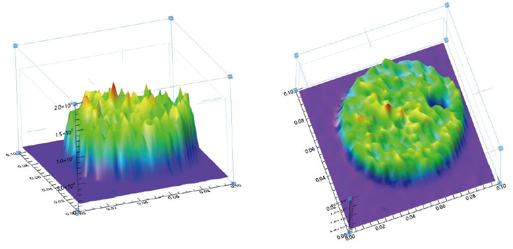
Fluorescence intensity image of a MicroLED microdisk (3D display):